FIFA 18 数据 - 俱乐部排名

2017 即将结束, FIFA 18 也早已发行. 我们可以来浏览一下 FIFA 18 的数据, 看看那些"最好"的俱乐部.

数据加载和预处理

首先从文末的链接下载 fifa 18 的数据文件, 然后加载:

import numpy as np
import pandas as pd
import seaborn as sns
import matplotlib.pyplot as plt

sns.set(style="white", color_codes=True)
fifa = pd.read_csv("./input/CompleteDataset.csv")
print(fifa.columns)

欧元文本类型转换

由于球员的身价和薪资数值是 string 类型, 比如 €5K , 所以文本的欧元需要转换为 number 类型:

def extract_value_from(value):
    if type(value) is float:
        return value
    out = value.replace('€', '')
    if 'M' in out:
        out = float(out.replace('M', ''))*1000000
    elif 'K' in value:
        out = float(out.replace('K', ''))*1000
    return float(out)

fifa['Value'] = fifa['Value'].apply(lambda x: extract_value_from(x))
fifa['Wage'] = fifa['Wage'].apply(lambda x: extract_value_from(x))

预处理完成后, 就可以进行一些聚合分析了.

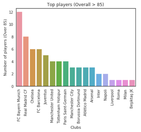
顶级球员最多的俱乐部

这里以 >= 85 分 作为顶级球员的定义, 来查询顶级球员最多的俱乐部.

cutoff = 85
players = fifa[fifa['Overall'] > cutoff]
grouped_players = players.groupby('Club')
number_of_players = grouped_players.count()['Name'].sort_values(ascending = False)

ax = sns.countplot(x = 'Club', data = players, order = number_of_players.index)
ax.set_xticklabels(labels = number_of_players.index, rotation='vertical')
ax.set_ylabel('Number of players (Over ' + str(cutoff) + ')')
ax.set_xlabel('Clubs')
ax.set_title('Top players (Overall > %.i)' %cutoff)
# seaborn using plt
plt.show()

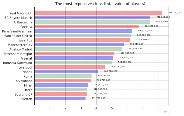
球员总身价排名

value_groupby_club = fifa.groupby('Club')[["Value"]].sum().sort_values(['Value'], ascending=[False]).head(20)
value_groupby_club.head()
fig = plt.figure(figsize=(8,6))
plt.title("The most expensive clubs (total value of players): ")
plt.yticks(np.arange(len(value_groupby_club.index.values)), value_groupby_club.index.values, fontsize=10)
plt.barh(np.arange(len(value_groupby_club.index.values)), value_groupby_club["Value"],align='center', alpha=0.4, color=['red', 'blue', 'g'])
plt.grid()
plt.gca().invert_yaxis()
plt.show()

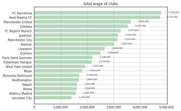
球员总薪资排名

fig = plt.figure(figsize=(8,6))
plt.title("total wage of clubs")
plt.yticks(np.arange(len(wage_groupby_club.index.values)), wage_groupby_club.index.values, fontsize=10)
plt.barh(np.arange(len(wage_groupby_club.index.values)), wage_groupby_club["Wage"],align='center', alpha=0.4, color='g')
plt.grid()
plt.gca().invert_yaxis()
ax = plt.gca()
import matplotlib
ax.get_xaxis().set_major_formatter(matplotlib.ticker.FuncFormatter(lambda x, p: format(int(x), ',')))
plt.show()

位置分类

将 Preferred Positions 中的位置进行一个大分类 (前中后):

positions = ['GK','CB','LCB','RCB','LB','RB','CM','LDM','RDM','CDM','CAM','LM','RM','ST','CF','LW','RW']
for p in positions:
    fifa['is' + p] = fifa['Preferred Positions'].str.match('.*[^a-zA-Z]*' + p + '[^a-zA-Z]*.*')
main_positions = ['Forward', 'Middle', 'Backward']
fifa['isForward'] = fifa['Preferred Positions'].str.match('ST|.*LW[^A-Z]+.*|.*RW[^A-Z]+.*|CF')
fifa['isMiddle'] = fifa['Preferred Positions'].str.contains('CM|LDM|RDM|CDM|CAM|LM|RM')
fifa['isBackward'] = fifa['Preferred Positions'].str.contains('CB|LCB|RCB|LB|RB|LWB|RWB')

把位置分好类之后, 就可以进行聚合分析了.

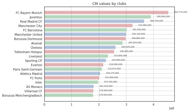
拥有中场球员价值

cm_groupby_club = fifa[(fifa['isMiddle']==True)] \
    .groupby('Club')[["Value"]].sum().sort_values(['Value'], ascending=[False])
cm_groupby_club = cm_groupby_club.head(20)

fig = plt.figure(figsize=(8,6))
plt.title("CM values by clubs")
plt.yticks(np.arange(len(cm_groupby_club.index.values)), cm_groupby_club.index.values, fontsize=10)
plt.barh(np.arange(len(cm_groupby_club.index.values)), cm_groupby_club["Value"], align='center', alpha=0.4, color=['r','g','b'])
for a,b in enumerate(cm_groupby_club["Value"]):
    plt.text(b-0.5, a, utils_conrrency_format(b), fontsize=7)
plt.grid()
plt.gca().invert_yaxis()
plt.show()

可以看到我大曼城排在第四.

对比平均身价

N = 3
length = 10
ind = np.arange(length)
width = 0.3
#
fifa['Value2'] = fifa['Value']
f_mean = lambda x: np.average(x, weights=fifa.loc[x.index, "Value2"])
f_agg = {'Value': [np.sum, "count"], 'Value2': {'ValueAvg' : f_mean} }
cm_groupby_club = fifa[(fifa['isMiddle']==True)].groupby('Club')[["Value", "Value2"]].agg(f_agg) \
    .rename(columns={'sum': 'Value'}).sort_values(['Value'], ascending=[False]).head(length)
cm_groupby_club = cm_groupby_club.head(length)
print(cm_groupby_club.columns)
print(cm_groupby_club)
club_st_higest_value = cm_groupby_club['Value'].max()
club_st_higest_wage = cm_groupby_club['ValueAvg'].max()
cm_groupby_club['ValuePercent'] = cm_groupby_club['Value'] / club_st_higest_value
cm_groupby_club['ValueAvgPercent'] = cm_groupby_club['ValueAvg'] / club_st_higest_wage

fig = plt.figure(figsize=(8,6))
ax = fig.add_subplot(111)
plt.title("middle values of clubs")
h1 = ax.barh(ind, cm_groupby_club["ValuePercent"], width, align='center', alpha=0.4, color='g')
for a,b in enumerate(cm_groupby_club["ValuePercent"]):
    ax.text(b - 0.2, a, utils_conrrency_format(b * club_st_higest_value), fontsize=7)
h2 = ax.barh(ind+width, cm_groupby_club["ValueAvgPercent"], width, align='center', alpha=0.4, color='r')
for a,b in enumerate(cm_groupby_club["ValueAvgPercent"]):
    ax.text(b - 0.2, a + width, utils_conrrency_format(b * club_st_higest_wage), fontsize=7)
ax.set(yticks=ind + width/2, yticklabels=cm_groupby_club.index.values, ylim=[2*width - 1, length])
plt.legend([h1, h2], ['Value', 'ValueAvg'])
plt.gca().invert_yaxis()
plt.show()

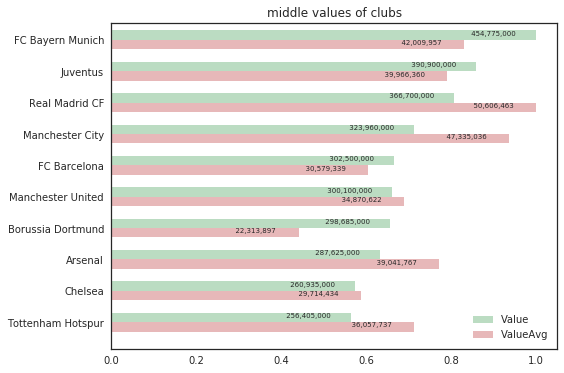
如图, 曼城的平均身价还是挺高的, 作为英超传控球队, 多储备优秀的中场球员有利于球队的发展.

拥有前锋球员价值

st_groupby_club = fifa[(fifa['isForward']==True)].groupby('Club')[["Value"]].sum().sort_values(['Value'], ascending=[False]).head(20)
st_groupby_club = st_groupby_club.head(20)

fig = plt.figure(figsize=(8,6))
plt.title("forward values of clubs")
plt.yticks(np.arange(len(st_groupby_club.index.values)), st_groupby_club.index.values, fontsize=10)
plt.barh(np.arange(len(st_groupby_club.index.values)), st_groupby_club["Value"],align='center', alpha=0.4, color=['g'])
for a,b in enumerate(st_groupby_club["Value"]):
    plt.text(b-0.5, a, utils_conrrency_format(b), fontsize=7)
plt.grid()
plt.gca().invert_yaxis()

plt.show()

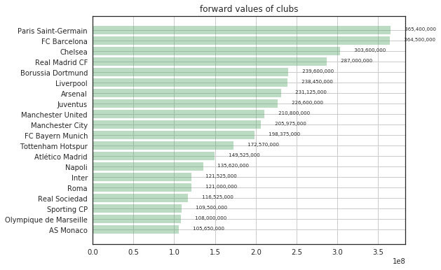
可以看到大巴黎夺冠, 这得感谢第二位巴萨的内马尔转会.

增加薪资水平对比

N = 3
length = 10
ind = np.arange(length)
width = 0.3

st_groupby_club = fifa[(fifa['isForward']==True)].groupby('Club')[["Value", "Wage"]].sum().sort_values(['Value'], ascending=[False]).head(length)
st_groupby_club = st_groupby_club.head(length)
club_st_higest_value = st_groupby_club['Value'].max()
club_st_higest_wage = st_groupby_club['Wage'].max()
st_groupby_club['ValuePercent'] = st_groupby_club['Value'] / club_st_higest_value
st_groupby_club['WagePercent'] = st_groupby_club['Wage'] / club_st_higest_wage
print(club_st_higest_value)
print(st_groupby_club)

fig = plt.figure(figsize=(8,6))
ax = fig.add_subplot(111)
plt.title("forward values of clubs")
h1 = ax.barh(ind, st_groupby_club["ValuePercent"], width, align='center', alpha=0.4, color='g')
for a,b in enumerate(st_groupby_club["ValuePercent"]):
    ax.text(b - 0.2, a, utils_conrrency_format(b * club_st_higest_value), fontsize=7)
h2 = ax.barh(ind+width, st_groupby_club["WagePercent"], width, align='center', alpha=0.4, color='r')
for a,b in enumerate(st_groupby_club["WagePercent"]):
    ax.text(b - 0.2, a + width, utils_conrrency_format(b * club_st_higest_wage), fontsize=7)
ax.set(yticks=ind + width/2, yticklabels=st_groupby_club.index.values, ylim=[2*width - 1, length])
plt.legend([h1, h2], ['Value', 'Wage'])
plt.gca().invert_yaxis()
plt.show()

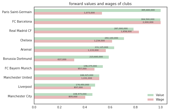
多特前场的薪资真低...

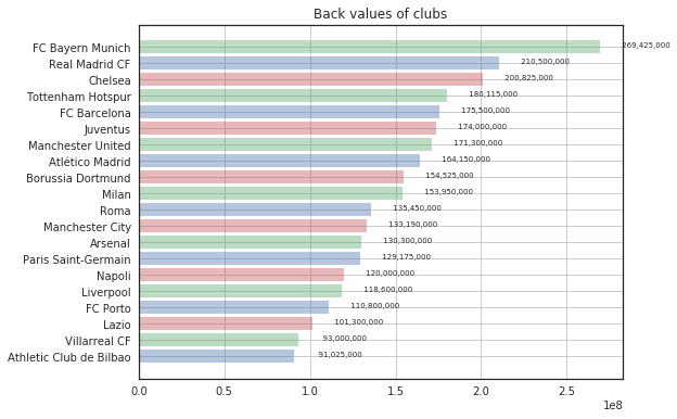
拥有后卫球员价值

back_groupby_club = fifa[(fifa['isBackward']==True)] \
    .groupby('Club')[["Value"]].sum().sort_values(['Value'], ascending=[False])
back_groupby_club = back_groupby_club.head(20)

fig = plt.figure(figsize=(8,6))
plt.title("Back values of clubs")
plt.yticks(np.arange(len(back_groupby_club.index.values)), back_groupby_club.index.values, fontsize=10)
plt.barh(np.arange(len(back_groupby_club.index.values)), back_groupby_club["Value"],align='center', alpha=0.4, color=['g', 'b', 'r'])
for a,b in enumerate(back_groupby_club["Value"]):
    plt.text(b-0.5, a, utils_conrrency_format(b), fontsize=7)
plt.grid()
plt.gca().invert_yaxis()
plt.show()

最后

---

这里只进行了一些简单的俱乐部分析, fifa 18 的数据还有许多待挖掘的地方,
比如潜力值/年龄/国度/更细的能力指标等, 有待大家去作出更多更好的可视化分析出来.
(以上数据都是基于 fifa 18 的数据, 和现实有一些差距的.)

参考

---

fifa 18 数据下载